From Data to Music – Pd as a Sonification Tool for Algorithmic Composition

Music is a physical phenomena: we can hear and sometimes feel sound waves, we can look at printed scores and chord charts and hold CD’s but these contain only a representation of musical information. How we represent music and each of the many musical characteristics is an important decision for the algorithmic composer. When creating algorithmic music we have to make choices about how we will represent musical information. This in turns impacts how we think about that musical information and affects what we can and cannot do with it.

Today’s algorithmic composition tutorial explores some of these issues and our algorithmic composition looks again at using sonification – a mapping of non-musical data to musical parameters to create an algorithmic piece of music. The key to sonification is how the data is mapped to musical parameters so in this post we’re using the same data with a more flexible interface that allows you to experiment with how the data is mapped to musical parameters.

Here’s a quick video demo of the Algorithmic Composition Sonification tool in action:
Here’s a breakdown of each of the sections, you can also download the patch at the end of the post.

If you haven’t already it’s worth reading through the previous sonification post, but as a quick recap here are the four basic steps of the sonification process:

1.            Find some interesting data
2.            Decide which musical parameters you want to map the data to
3.            Fit the input data to the correct range for your chosen musical parameters (normalise)
4.            Output remapped data to MIDI synths, audio devices etc

Step 1 involves sourcing some interesting data.
Ideally the data you use should include some patterns as this tends to result in more satisfying compositions. In this patch we’re using the same weather data as in the previous algorithmic composition post, but in a future post we’ll include the facility to load up data from any .csv file.

Step 2, involves deciding how you will map your data to musical parameters e.g. pitches, frequencies, rhythms, dynamics, timbre etc. The example patch today allows you to experiment with different mappings ‘on the fly’ and instantly hear the result. You can then save the mappings you like as presets.

Step 3 involves scaling the input data to match the output range you want. For example in our data temperature ranges from 6.6c to 20.6c. If we wanted to map this to a range of MIDI notes we would need to rescale the data so that the output data fitted into the number range we wanted e.g. changing 6.6 and 20.6 to one octave of MIDI notes from middle C, MIDI note 60 to 72.

Step 4 involves connecting the rescaled numbers from our source data to an output of our choice, typically a synth, MIDI device or audio processor.

Choosing Musical Parameters Pitch
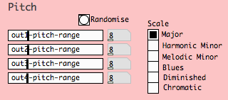
The pitch section of this sonification patch allows you to choose a scale that the data will be mapped to and a pitch range. In this screenshot the data has been mapped to 8 notes (one octave) of a major scale. Here four sliders allow you to set each part to a different pitch range.



Changing the pitch range will keep the same contour shape as the original data but will map the data across a wider or narrower range. In this chart for example, the same set of data has been remapped to different ranges, although the contour follows the same shape as the original data, if mapped to pitch the melodies would span different pitch ranges.

Increasing the pitch range that the data is mapped to exaggerates the contours of the melody creating higher peaks and lower troughs, decreasing the pitch range will result in a melody with smaller intervallic steps.

This allows us to create many different musical examples from the same set of source data. The incoming data is normalised to the selected pitch range using an expression.

It’s worth noting that when mapping to a scale that unless you’re mapping to a chromatic scale or whole-tone scale, each of the scale intervals are not equal (e.g. a major scale being constructed of semitone intervals 2, 2, 1, 2, 2, 2 1), this would slightly distort the interval steps present in the original data.
Scales are selected using the radio buttons.


The scales are stored in tables that are accessed by a tabread object.

As well as mapping the data over a pitch range, we also need to decide the base pitch for each of our four musical parts. Using radio buttons we can choose the octave for each part individually and an overall transposition factor.

The selected base pitch is added to the scale note and added to a transposition number.

Rhythm Tempo Factor
The tempo factor controls the speed of each part. With a tempo factor of 1 the part will run at normal speed. At .5 it will run at double speed, at 2 it will be at half speed etc. The link_tempo/octave toggle allows you to link the tempo and octave so that faster parts will be played at higher octaves and slower parts at lower octaves. The tempo factor can be randomised.

The staccato/legato factor controls the note length in relation to the tempo. Lower values will give short staccato notes, higher values will give longer legato notes. The tempo is set here.

Dynamics: Random Velocity Range and Channel Mixer
In this example the MIDI velocities are randomised rather than mapped to the sonification data. The range of possible velocities is set using these sliders and can also be randomised.

The mixer offer a simple way of adjusting the relative level of each part, these levels can be randomised using the bang button.

MIDI program numbers for each part can be changed by scrolling or typing in the number boxes, the GM instrument name will then be shown in the corresponding symbol. The MIDI program number can be also be randomised.

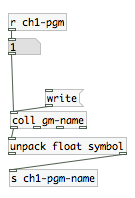
The MIDI program names are stored in a coll object, entering a number looks up the appropriate index of the coll and this name is sent to the symbol.

Save and Recall Presets
Values for the whole patch can be stored and recalled as presets. Choose a preset number to save or recall and press the appropriate bang button.

You can download the PureData sonification patch here.
There will be a Max version posted shortly and a more extended version that allows you to easily load up your own data and remap it to different parameters. Check out the algorithmic composition forum to introduce yourself and ask any questions, check back soon and keep composing!