Showing posts with label tutorial. Show all posts

Tuesday, 12 January 2016

Sonification - Algorithmic Composition


Today's algorithmic composition tutorial uses sonification as a composition tool. Sonification uses data that is typically not musical and involves remapping this to musical parameters to create a composition. 

Sonification can be used to hear information in a set of data that might be otherwise difficult to perceive, common examples include Geiger counters, sonar and medical monitoring [ECG]. When creating sonification algorithmic compositions we are interested in creating interesting or aesthetically pleasing sounds and music by mapping non-musical data directly to musical parameters.

Here is some example output:


The Sonification Process:
There are four simple steps involved in creating a sonification composition.
1.            Find some interesting data
2.            Decide which musical parameters you want to map the data to
3.            Fit the input data to the correct range for your chosen musical parameters (normalise)
4.            Output remapped data to MIDI synths, audio devices etc

Step 1 – Find an interesting set of data
First of all we need to source a data set. You can use any data you like stock markets, global temperatures, population changes, census data, economic information, record sales, server activity records, sports data - any set of numbers you can lay your hands on, here are some possible sources: Research portal, JASA data, UK govt data
 
It's important to select your source data carefully. Data that has discernable patterns or interesting contours works particular well for sonifications. Data that is largely static and unchanging will not be interesting, similarly data that is noise-like is usually of limited use.

Here we've loaded some example data into a coll object in PureData

And similarly in Max:

algorithmic composition maxmsp sonification

Step 2 - Map Data to Musical Parameters
The second step is the most creative of the sonification process. It involves making creative decisions about which musical parameters to map the data to e.g. pitch, rhythm, timbre and so on. 

This is more of an involved question than it initially appears, if we choose to map our data to pitch, we also have to choose how these pitches will be represented:
 
Frequency (20Hz - 20kHz): this is useful for direct control of synths, filter cutoffs etc, but is not intuitively musical and typically needs conversion if working with common musical scales
MIDI notes (0 - 127): assumes 12 note division of the octave, no representation of C# versus Db
MIDI cents
•    OpenMusic uses a MIDIcents representation. This is equivalent to MIDI notes * 100 so middle c is 6000
•    This enables microtonal music and alternative divisions of the octave, for example dividing the octave into 17.
Pitchclass
•  octaves are equivalent
Scale degree
•    Assumes use of a scale and returns the degree of that scale.
•    This is useful as we can easily deal with uneven steps in the scale simply

Step 3 – normalise data to fit musical parameters
In Max we can use the scale object. Scale maps an input range of float or integer values to an output range. The number is converted according to the following expression
 y = b e-a c x  c

where x is the input, y is the output, a, b, and c are the three typed-in arguments, and e is the base of the natural logarithm (approximately 2.718282).


expr $f4 + ($f1 - $f2) * ($f5 - $f4) / ($f3 - $f2 )
1 = number
2 = input min
3 = input max
4 = output min
5 = output max

Step 4 – Output
Adding in some MIDI objects allows us to hear our data sonified in a simple way:
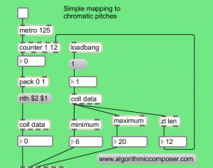
algorithmic composition sonification maxmspAnd in PureData adding in a makenote and noteout objects and normalising our output data to one octave of a chromatic scale looks like this.sonification puredata algorithmic composition
You should now have some basic musical output to your MIDI synth. Now the patch is setup it’s easy to experiment with mapping the data to different pitch ranges. For example:
  • Try adjusting the normalisation (the scale object in Max or expr object in PureData) to map the data across two octaves instead of one by changing the output range from 12 to 24 – or any other pitch range.
  • The + 60 object sets our lowest pitch as MIDI note 60, this can be modified easily to set a different pitch range.
  • Invert the data range by having a high output minimum and a lower maximum, so ascending data creates descending melodic lines.
Mapping to Scales
As an alternative to mapping our data to chromatic pitches we can use a different pitch representation and map our scale to the notes of a diatonic scale.
First we need to define a few scales in a table in Max:
sonfication algorithmic composition maxmsp
As the contents of tables are defined slightly differently in PureData this looks like this:
sonification algorithmic composition puredata
The above screenshots show the scale intervals for a Major, Harmonic Minor, Melodic Minor and Natural Minor scale being stored in a separate table for each scale. These are stored as pitchclasses, if we need to transpose or modulate our composition to another key we can add or subtrack to these scale notes before the makenote object e.g. to transpose up a tone to D add a + 2 object. Now rather than mapping to chromatic pitches we’ll map to scale pitches so we’ll need to modify our normalisation to reflect this.
sonification puredata algorithmic composition
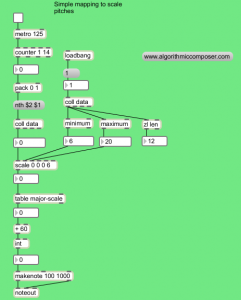
Here we’ve changed the output range to be 0 to 6 to reflect the seven different scale degrees of the major scale. Similarly in Max:
sonification maxmsp algorithmic composition
We are now mapping our octave to a major scale, as we have already stored a number of scales you could try changing the name of the table that is being looked up to map to an alternative scale e.g. table harmonic-minor-scale.
We can also map the data to a scale over more than one octave.
sonification algorithmic composition puredata
Here we’ve changed the output range in this example to be 0 to 20. Using % (modulo) to give us the individual scale degrees and / (divide) to give us the octave. The process is the same in Max, although in the previous example we mapped across 3 octaves of the scale there’s no requirement to map to full octaves, you could map your data to 2 1/2 octaves or any other pitch range by changing the output values of the scale object (expr in PureData):
sonification algorithmic composition maxmsp
So far we have mapped our data to MIDI pitches. The next example maps the data to frequencies and uses this to control the cutoff frequency of a band pass filter that is fed with noise. This gives a sweeping windsound effect.
As an alternative to MIDI output we’ll map our wind data to the filter cutoff of a bandpass filter that is fed with noise. As we’re know working with frequencies rather than MIDI notes we’ve changed the output of the scale object to remap any incoming data between 200Hz and 1200Hz:
algorithmic composition maxmsp sonification
The patch is setup in a very similar way in PureData with a bp~ object as our band pass filter, rather than the reson~ object found in MaxMSP.
puredata algorithmic composition sonification
Although all of the notes are created by mapping the data directly to pitches we have made another of creative decisions along the way, so there are many ways of realising different sonifications of the same source data. So far we have only mapped to pitch however we still have a number of variables we can alter:
scale – chromatic, major, melodic minor, natural minor, harmonic minor (any other scales can be defined easily)
base pitch (the lowest pitch )
pitch range (range above our lowest pitch e.g. 2 octaves)
the data set used to map to pitches
As with any composition we also have to make musical decisions concerning which instrument plays when, timbres and instrumentation, dynamics, tempo etc. In another post we’ll look at sonifying these elements from data but for now we’ll make these choices based on aesthetic decisions.
Summary
In the youtube example we have added several copies of the sonification patch so we have one for each of our data sets (temperature, sunshine, rainfall and windspeed). The interesting thing about using weather data is that we should hear some relationship between the four sets of data.
We’ve also added a score subpatch with sends and receives to turn on and off each section and control the variables mentioned above (min pitch, pitch range etc).
After the getting the patch to work play around with your own settings and modifications and check out part two of this sonification algorithmic composition tutorial. Future posts will continue the idea of mapping and explore sonifying rhythm, timbre and other musical parameters. Have fun and feel free to post links to your sonification compositions below.
Post a comment if you’ve any questions on this patch.

Tuesday, 16 August 2011

Tom Johnson's Algorithmic Compositions Part 2

A previous post looked at some of the algorithmic composition ideas used by American Composer Tom Johnson. Today's algorithmic composition tutorial looks at a few more of Johnson's concepts specifically his use of finite automata.

A finite automaton is a sequence using a finite number of symbols generated according to specific rules. In the case of Johnson's Automatic Music, six percussionists each have only two notes, high and low, and the alphabet is limited to 1 (the low note), 2 (the high note), and 3 (a silence) using the following rules:

1 --> 1 1 2
2 --> 3 2
3 --> 3 3

Beginning with 1 generates the following sequence:

   112112321121123233321121123211211232333233333332

Using this automaton it's easy to generate long sequences of numbers that can be then mapped to musical parameters. As ever with algorithmic composition, once you've created your patch or program it's easy to manipulate the formula or remap the musical output to generate new pieces.

Let's have a look at a simple example using PureData and Max. This screenshot shows the generation part of our algorithm in PureData.

The until object will output 500 bangs when the above message is clicked on, the counter outputs a running count of these bangs and this is used as a number to lookup the stored value in the coll object. The output of the coll is connected to a select object and this triggers the new messages that are stored within our coll object.

In Max the patch looks very similar though note the use of Uzi rather than the PureData until object.

Monday, 27 June 2011

Tom Johnson's Self Similar Melodies

The American Composer Tom Johnson often uses simple mathematical principles in his compositions. Today's algorithmic composition tutorial looks at a few of Johnson's algorithmic concepts and applies them using Max and PureData. As Max and PureData use slightly different objects to read and write data from tables we'll include screenshots of the algorithmic composition patches from both applications.

Self Similar Melodies
This first example taken from Johnson’s now out of print book ‘Self Similar Melodies’ makes use of the following expression:

                        n             n+1            n-1             n

Inputting a zero into our algorithm gives us the following four numbers:

                        0            1            -1            0

It’s easy to apply this in PureData:

and in Max:


Second Order Markov Chains in PureData

It's been too long since the last algorithmic composition post, but a series of new posts are on the way!

To kick things off we'll revisit one of our previous Markov chain algorithmic compositions. Previously we looked at first order Markov chains in PureData. We also extended this into a second order Markov chain in Max.

Let's have a quick recap first.

First Order Markov Chains
In a previous Algorithmic Composition post we built a first order Markov Chain analysis and generation patch. In 1st order Markov chains the next note is based on the current note and a list of probabilities for following notes. This is stored in a State Transition Matrix (STM), here's an STM that lists the notes of Happy Birthday and the probabilities of each subsequent note.


Second Order Markov Chains
Second order Markov Chains choose the next note based on the two previous notes and the probability of subsequent notes following those two notes:

Sunday, 23 May 2010

Algorithmic Composition with timbres: Klangfarbenmelodie

Algorithmic composition often tends to focus on pitch and rhythm. Today's algorithmic composition tutorial concentrates on timbre, creating algorithmic music by outputting MIDI from MaxMSP [Max] and PureData [PD].

Klangfarbenmelodie (German for tone color melody) and the synonymous French term mélodie de timbres distributes a melody over several instruments rather than assigning it to just one, the listener's focus becomes timbre rather than pitch.

In a similar way, the algorithmic composition patch we'll build today outputs series of overlapping randomly chosen timbres to create an interesting musical texture.

Jump to the end of the post to hear some sample algorithmic music output from this patch.

Algorithmic Composition with MIDI Timbres
Firstly we'll get a simple MIDI note to play in Max and PureData: add a toggle, a metronome object, a message and makenote and noteout objects. If you're not sure how to do this, work through some of the earlier algorithmic composition tutorials here:
Your Max or PureData patch should now look like this, you should also hear a MIDI note when you turn the toggle on. If not, check you have a MIDI output device selected.
algorithmic composition with timbre Max 1algorithmic composition with timbre PureData 1

Saturday, 8 May 2010

Algorithmic Composition: Markov Chains in PureData

We've looked at Markov Chains in a few previous Algorithmic Composer tutorials including Markov Chains in Keykit and Markov Chains in OpenMusic. Today we'll be creating some algorithmic music by composing with Markov Chains in PureData.


Markov Chains choose the next state based on the current state and a set of probabilities. Mapped to pitch this would involve choosing our next note based on our current note and a list of possible next notes and their probabilities.

In today's tutorial we'll look at examples of Markov Chains and use them to generate pitches for a simple algorithmic composition.

Sunday, 2 May 2010

Algorithmic Composition | OpenMusic Rhythm Trees Tutorial Part 1

In previous algorithmic composition tutorials we've looked at using OpenMusic for algorithmic composition, today's algorithmic composition tutorial introduces Rhythm Trees.

Rhythm trees are a way of representing rhythm with nested lists. The notation can get quite unwieldy and a little complicated, however these disadvantages are outweighed by the advantages. using rhythm trees it's possible to represent very complex rhythms with relatively simple notation, it's also possible to create simple and complex rhythms using algorithmic composition techniques.

The simplest way to work with rhythm trees is to enter a list of rhythms and connect this to the tree input of a voice object.

Friday, 30 April 2010

Random Walks in Max and PureData

It's been a while since we've looked at PureData and Max as algorithmic composition tools, today's algorithmic composition tutorial looks at Random Walks.

We've looked before in this Random Walks OpenMusic tutorial but this is the first time we've used in random walks in Max and PureData.

Random Walks
We'll start with a simple example:

1. Given a starting pitch of middle C
2. We will make a random choice of two possibilities, up or down 1 semitone from our current pitch
3. We now have a new pitch, from this new pitch go back to step 2 and repeat.


The easiest way to use random walks in Max and PureData is to use the drunk object. This object allows you to set a start value, maximum step size and a bound. Drunk then performs a random walk between 0 and the bound value. Here's an example of a drunk random walk in PureData:


And in Max:

Sunday, 25 April 2010

OpenMusic and Chaos - OMChaos library

Our last few Algorithmic Composition posts have featured OpenMusic tutorials. We're continuing our look at OpenMusic today by looking at chaos, using the OMChaos library.

Chaos theory is a field of mathematics where dynamic systems are very sensitive to initial conditions. The famous 'butterfly effect' states that small differences can lead to large variations later: the small flap of a butterfly's wings may cause effects that later alter the path of a tornado.

Many of our previous algorithmic composition tutorials have used random elements (e.g. probabilities and Markov chains). Although Chaos might appear random, it's important to note that it is deterministic: if you run the algorithm again with exactly the same input it will produce the same output.

Today we'll start to look at using some Chaos algorithms to generate algorithmic music.

OpenMusic and Chaos - The OMChaos library
1. Make sure that OMChaos has been enabled in the preferences of OpenMusic.


2. Create a new patch in your workspace. OMChaos has 4 categories of functions: orbitals, IFS, fractus and UTILS.


3. The OMChaos orbitals menu features the core of the library. Each of these orbitals functions is a different chaos algorithm. Each of them shares the important chaos algorithm characteristic: small changes in initial conditions can lead to large changes later.

4. We'll start by using the KAOSN function.

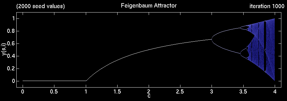
5. This OpenMusic function is a form of a very common chaos algorithm fn+1=cfn(1-fn). That's to say: to get the next value of f, multiply the current values of c, f and (1 - f). This formula involves only 1 subtraction and two multiplies but it leads to chaotic behaviour. In this graph you can see with values of c below 3 the behaviour is very predicatable. However if c > 3.75 then very small changes in f lead to very large changes later on:


6. Here we've used 24 values for .95 for f 3.75 for c and set the length to be 24. Evaluating the KAOSN function will produce a series of 24 values based on these input parameters. Each time its evaluated it will produce the same numbers. If we change the input values to f 3.75 and c .94999, the numbers generated will start the same but slowly deviate as the sequence grows in length: the butterfly effect, small changes in initial conditions lead to large changes later on.


7. We'll use this chaos function to generate pitches between MIDI note 48 and 72. The output of the kaosn function is a series of floating point numbers between 0 and 1. To get the number in the range we want add:
  • an om* function and 24, giving our series a range of 0 to 24
  • an om+ function and 48 giving our series a range of 48 to 72
  • an om* function and 100, to change MIDI notes into the MIDIcents pitch representation OpenMusic uses
  • The om-round function rounds these numbers into integers

8. In this patch we'll have two voices with slightly different initial conditions for our chaos function. They will start playing identical notes and then slowly start to deviate. We'll append a reversed copy of the list, so we'll have a musical palindrome. To do this we can add cons and reverse functions. Reverse will reverse our original pitch list and cons will add this reverse pitch list to the end of our original pitch list. If you evaluate the cons function you'll see it's created list of lists (two sets of parentheses), we use the flat function here to flatten the list into a single set of parentheses:


9. Connect the output of voice, to the chords input of a voice.

10. We now need to duplicate what we have so far so we can create another set of pitches with slightly a different initial for our KAOSN function. Select all [CMD A on Mac, CTRL A on PC] and duplicate [CMD D on Mac, CTRL D on PC]. Change the second input to one your KAOSN functions to .94999, so that the two sections have slightly different initial conditions.

11. We also need to tell OpenMusic what rhythm to use for our melody. The voice function uses Rhythm Trees as its rhythmic representation. Rhythm trees are beyond the scope of this algorithmic composition post, but we will create some algorithmic music with rhythm trees in a future algorithmic composition tutorial. For now add in a repeat-n function and a mktree function. In this example we'll create 48 32nd notes:


10. Your patch should now look something like this (click on the image for a larger version):
11. To evaluate each voice press v, to play the voice press p to send it to a MIDI port. If you haven't done this already you can set up your MIDI outputs in OpenMusic preferences.

12. To hear both voices at the same time we need to create a list of both voices add in a poly function.


13. We can now hear both voices starting with the same pitches, slowly diverging and the converging back to the same pitches.

14. We'll be looking at rhythm trees in more detail in a future post, but for now to make the rhythms more interesting we'll use the nth-random function to choose randomly from a list of possible rhythms: (1/32 1/8 -1/16 -1/4 1/16) negative numbers represent rests. Repeat-n will generate a hundred of the randomly chosen rhythms:
15. Your final patch should look like something like this (I've changed the length of the sequence for both KAOSN functions to 50, giving us a melody 100 notes long when the reversed melody is added to the end). Click on the image for a larger version.


OpenMusic OMChaos Library Tutorial Summary
We've created an OpenMusic patch using the OMChaos library to generate chaotic pitches. Two voices have been used, with slightly different initial conditions the melodies diverge. Appending a reverse version of the melody on the end gives us a musical palindrome.

We then introduced the concept of rhythm trees in OpenMusic and randomly selected some rhythms from a given list.

Subscribe to the RSS feed and tune back regularly for more algorithmic composition tutorials, posts and reviews using Common Music, OpenMusic, PureData, MaxMSP and other algorithmic composition software.

Friday, 23 April 2010

OpenMusic Markov Chains and omlea

We've looked at using OpenMusic for algorithmic composition in a number of posts before, we've also looked at using the OpenMusic OMalea library and random walks in OpenMusic. Today we're going to use OpenMusic and OMalea to work with Markov Chains.

Markov Chains are a very useful tool for the algorithmic composer, we've looked at Markov Chains in keykit here. If you're not familiar with how Markov Chains work it's definitely worth reading this algorithmic composition post.

In brief, Markov Chains chose the next note using a probability. For example if the current note is E, there might be a 70% chance of the next note being a A and a 30% chance of it being an C#. These probabilities are stored in something called a transition table or transition matrix.

We can either create the transition matrix by hand or we can create it by analysing an existing piece of music (or any other piece of data).


This is the approach we'll take in today's post. We'll load up a MIDI file, create a transition matrix from this using the ana-mark function, and then generate new melodies based upon this.

1. First of all we need to load up a MIDI file. Create a new class MIDIfile, either by choosing from the menu or CMD clicking (CTRL click on PC) and typing midifile.


2. Evaluate the midifile class by hitting the 'v' key or CMD clicking on it's output (CTRL click on PC). This will allow you to load up a MIDI file, once it's loaded make sure the midifile class is selected and press b to lock it. This will ensure that you don't have to load the MIDIfile every time you evaluate the patch.

3. We next have to extract the pitch data from the MIDI file. We can also use markov chains to generate rhythm, dynamics and other musical information, but for now we'll stick with pitch. Add a mf-info function, this allows to extract each note from the MIDI file.

4. If you evaluate the mf-info function, you can see a list of lists that describe each note, something like this, where the values are pitch, onset, duration, velocity and MIDI channel
((64 1000 500 52 1) (73 1500 385 58 1) (74 1875 125 43 1) (62 2000 500 32 1))

5. We need to access just the first element of each set of parentheses: the pitch. There are a number of ways we can do this, but the simplest is to use the mat-trans function followed by the first function. Add these in one a time and evaluate them to see what they do. You patch should now look like this:


6. Now when we evaluate our patch we get a list of pitches. This can be fed into the ana-mark function (remember you need the omalea library enabled to be able to use this function - this can be turned on in preferences if it's not already).

The ana-mark function in OpenMusic automatically generates a Markov transition matrix for us of the form:
((list-of-pitches ((first-pitch-probabilities) (second-pitch-probabilities... ... (last-pitch-probabilities)))

Something like this:
((1 2 3) ((0.0 1.0 0.0) (0.333 0.0 0.667) (0.0 1.0 0.0)))

7. We need to be able to separate our list of pitches, the first element in the list [ (1 2 3) in the above example ] from the list of probabilities [the second element in the list]. For this we can use the Lisp functions first and second. You can type first and second directly into a new box to create them, or create them from the drop down menu. So far our patch looks like this:

8. We can now connect a Markov function. There are two Markov functions in the OpenMusic omalea library, markov1 generates a single next pitch and can be used with repeat-n to generate a series of pitches. Markov2 generates a series of pitches. Here we've added a markov2 function and asked it to create a series of 50 notes starting with the first note.

9. When you evaluate markov2 you'll notice that outputs the index rather than the actual pitch we entered. So if we were using notes 60, 64, 65 and 67 the markov2 function thinks of them as 1, 2, 3 and 4. We can easily map this index to our original list of pitches by using the posn-match function (position match). Your finished patch should look like this:
Now when you evaluate the patch, we generate a list of pitches based upon the original set of pitches in out MIDI file. To get a better understanding of what's happening at each stage, evaluate each function in turn by selecting and pressing v and looking at the output in the listener window. To get a better understanding of Markov Chains in general do have a read through a previous on Markov chains and algorithmic composition.

You can also try using the Markov chains to generate elements of your CSound scores as looked at in the post on algorithmic composition, OpenMusic and CSound - using the om2csound library.

Check back soon for more algorithmic composition techniques and tutorials.

Friday, 16 April 2010

Probabilities in OpenMusic using OMalea

We've introduced OpenMusic the computer-aided composition environment in a couple of previous algorithmic composition posts.

Today we'll have a look at using the OpenMusic library omalea to discuss the concept of probabilities and music. OpenMusic has a number of libraries that give additional functionality. Omalea (OM stands for OpenMusic and alea is Latin for dice. Aleatoric music uses chance as part of the compositional process. Both Pierre Boulez and John Cage have made use of aleatoric processes).

To enable the omalea library, go to preferences:

Check the omalea checkbox to load and enable the library:

In your workspace, create a new patch.
The omalea library offers four categories of functions: distributions, alea-seq, random-walk and tools.

Distributions
The distributions functions offer a range of ways of making aleatoric choices with different probability distributions.
The range of distributions includes linear (each possibility has the same chance of being selected e.g. RAN and RAN01), through choosing between 2 or a set a number of possibilities where you define their probability of being selected (CHOIX and CHOIXMULTIPLE), through to various triangle and various bell curve like distributions.

Choices (choix) - a coin flip' between two choices where you can adjust the probability. Here it's set to 50/50 chance of being note 5900 (B) and 6200 (D) - OpenMusic using MIDIcents to represent pitch so middle C (MIDI note 60) is 6000.

Poisson - a bell curve of normal distribution based around MIDI note 60.

A linear distribution.
When using the distribution functions to create pitches we had to perform a number of other operations to scale the numbers up and get appropriate values. OpenMusic uses MIDIcents to represent pitch so 6000 = MIDI note 60 or middle C.

If we're creating pitches, it's probably easy to use the alea-seq functions:


Not-centr chooses a random pitch, in this example around note 6000 +/- 12 semitones. It chooses only one value, here the repeat-n function has been used to generate a list of 8 randomly chosen notes:
Alea-seq works in a similar way, however as you can see in this example, it can generate lists of notes. Here we generate 8 notes, there's no need for the repeat-n function if using this object:
Linea-seq also produces a sequence of notes with a linear distribution. Using linea-seq you specify the number of notes and the upper and lower boundaries:


Triang-seq works in the same way to linea-seq, however it uses a triangle distribution. Notice how the notes are more centred around middle C:


Randomness, probabilities and chance are very useful tools for algorithmic composers. We'll look at these more in future posts in both OpenMusic and other software. We'll also have a look at some of the remaining omalea functions in future http://www.algorithmiccomposer.com/ posts and start to pull the tools together to create full compositions.