From Data to Music – Max as a Sonification Algorithmic Composition Tool

Music is a physical phenomena: we can hear and sometimes feel sound waves, we can look at printed scores and chord charts and hold CD’s but these contain only a representation of musical information. How we represent music and each of the many musical characteristics is an important decision for the algorithmic composer. When creating algorithmic music we have to make choices about how we will represent musical information. This in turns impacts how we think about that musical information and affects what we can and cannot do with it.

Today’s algorithmic composition tutorial explores some of these issues and our algorithmic composition looks again at using sonification – a mapping of non-musical data to musical parameters to create an algorithmic piece of music. The key to sonification is how the data is mapped to musical parameters so in this post we’re using the same data with a more flexible interface that allows you to experiment with how the data is mapped to musical parameters.

Here’s a quick video demo of the Algorithmic Composition Sonification tool in action:

All of the musical examples are different mappings of the same 12 months of weather data. Here’s a breakdown of each of the sections, you can also download the patch at the end of the post.

If you haven’t already it’s worth reading through the previous sonification post, but as a quick recap here are the four basic steps of the sonification process:

1. Find some interesting data
2. Decide which musical parameters you want to map the data to
3. Fit the input data to the correct range for your chosen musical parameters (normalise)
4. Output remapped data to MIDI synths, audio devices etc

Step 1 involves sourcing some interesting data.
Ideally the data you use should include some patterns as this tends to result in more satisfying compositions. In this patch we’re using the same weather data as in the previous algorithmic composition post, but in a future post we’ll include the facility to load up data from any .csv file.

Step 2, involves deciding how you will map your data to musical parameters e.g. pitches, frequencies, rhythms, dynamics, timbre etc. The example patch today allows you to experiment with different mappings ‘on the fly’ and instantly hear the result. You can then save the mappings you like as presets.

Step 3 involves scaling the input data to match the output range you want. For example in our data temperature ranges from 6.6c to 20.6c. If we wanted to map this to a range of MIDI notes we would need to rescale the data so that the output data fitted into the number range we wanted e.g. changing 6.6 and 20.6 to one octave of MIDI notes from middle C, MIDI note 60 to 72.

Step 4 involves connecting the rescaled numbers from our source data to an output of our choice, typically a synth, MIDI device or audio processor.

Choosing Musical Parameters Pitch
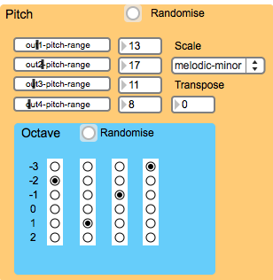
The pitch section of this sonification patch allows you to choose a scale that the data will be mapped to and a pitch range. In this screenshot the data has been mapped to 8 notes (one octave) of a major scale. Here four sliders allow you to set each part to a different pitch range.


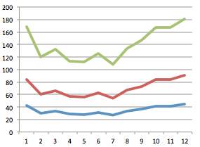
Changing the pitch range will keep the same contour shape as the original data but will map the data across a wider or narrower range. In this chart for example, the same set of data has been remapped to different ranges, although the contour follows the same shape as the original data, if mapped to pitch the melodies would span different pitch ranges.

Increasing the pitch range that the data is mapped to exaggerates the contours of the melody creating higher peaks and lower troughs, decreasing the pitch range will result in a melody with smaller intervallic steps.

This allows us to create many different musical examples from the same set of source data. The incoming data is normalised to the selected pitch range using an expression.



It’s worth noting that when mapping to a scale that unless you’re mapping to a chromatic scale or whole-tone scale, each of the scale intervals are not equal (e.g. a major scale being constructed of semitone intervals 2, 2, 1, 2, 2, 2 1), this would slightly distort the interval steps present in the original data.
Scales are selected using the umenu object.


The scales are stored in tables that are accessed by a tabread object.

As well as mapping the data over a pitch range, we also need to decide the base pitch for each of our four musical parts. Using radio buttons we can choose the octave for each part individually



A number box is used modulate all four parts, transposing to a new key.



The selected base pitch is added to the scale note and added to a transposition number.


Rhythm Tempo Factor
The tempo factor controls the speed of each part. With a tempo factor of 1 the part will run at normal speed. At .5 it will run at double speed, at 2 it will be at half speed etc. The link_tempo/octave toggle allows you to link the tempo and octave so that faster parts will be played at higher octaves and slower parts at lower octaves. The tempo factor can be randomised.

The staccato/legato factor controls the note length in relation to the tempo. Lower values will give short staccato notes, higher values will give longer legato notes. The tempo is set here.


Dynamics: Random Velocity Range and Channel Mixer
In this example the MIDI velocities are randomised rather than mapped to the sonification data. The range of possible velocities is set using these sliders and can also be randomised.


The mixer offer a simple way of adjusting the relative level of each part, these levels can be randomised using the bang button.

MIDI program numbers for each part can be changed by scrolling or typing in the number boxes, the GM instrument name will then be shown in the corresponding symbol. The MIDI program number can be also be randomised.


The MIDI program names are stored in a coll object, entering a number looks up the appropriate index of the coll and this name is sent to the symbol.

Save and Recall Presets
Values for the whole patch can be stored and recalled as presets, this is much easier to implement in Max than Pd. Click on a preset to recall it or shift click to store.


You can download the Max version of this patch here.

You can find the PureData sonification tutorial patch here. An extended version of this sonification patch that allows you to easily load up your own data and remap it to many more parameters will be posted shortly. Post a comment if you’ve any questions on this patch.

Tone Rows - PureData and Max

Today's algorithmic composition tutorial looks at manipulating a tone row in Max and PureData to generate musical material. We'll also have a look at one technique that's useful in generating more fully formed compositions in Pd and Max than some of the musical sketches we've generated so far.

Jump to the end of the post to hear some sample algorithmic music output from this patch.

As with yesterday's OpenMusic tutorial we're using the tone row from Berg's Violin Concerto:

  G, Bb, D, F#, A, C, E, G#, B, C#, Eb, F

You can use any tone row of your choosing. To start with we'll define our tone row in a table in PureData

and in Max

We'll start simply by playing through the tone row. As Max and PureData read and write to tables in slightly different ways the patches are setup a little differently in each. In Max the table object is used to read the table data:

Open Music - Tone Rows and the Maquette

Today's algorithmic composition tutorial looks at using OpenMusic to manipulate and generate musical material from tone rows.

If you haven't already got OpenMusic 6.5 installed you can download OpenMusic free for Mac and PC here. IRCAM supply a number of tutorials but you can also look through the OpenMusic tutorials available here.

Jump to the end of the post to hear some sample algorithmic music output from this patch.

Serialism developed as a framework for composing and organising atonally and moves away from the sense of a key by giving each pitch equal worth. This patch starts with a tone row from the Berg Violin Concerto:

   G, Bb, D, F#, A, C, E, G#, B, C#, Eb, F

All pitches must be played through in order, in order to provide more melodic material the tone row can be transposed to any pitch, inverted and played backwards.

First we'll create our tone row (to create a new object CMD click and type in to the box created).

Chaos in Max and PureData

We've looked at a few algorithmic composition ideas using Chaos in OpenMusic here, today's post applies some of these ideas algorithmic composition ideas in Max and PureData.

Chaos theory is a field of mathematics where dynamic systems are very sensitive to initial conditions. The famous 'butterfly effect' states that small differences in initial conditions can lead to large variations later: the small flap of a butterfly's wings may cause effects that later alter the path of a tornado.

As with our OpenMusic chaos patch, for this example of Chaos in PureData and Max we'll use a logistic map. The Logistic Map is a simple example of a discrete dynamical system that actually names a whole family of iterative functions described by the very common Logistic Equation:

f_n+1=cf_n(1-f_n)

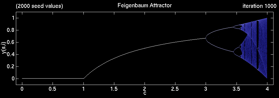
That's to say: to get the next value of f, multiply the current values of c, f and (1 - f). This formula involves only 1 subtraction and two multiplies but it leads to chaotic behaviour. In this graph you can see with values of c below 3 the behaviour is very predicatable. However if c > 3.75 then very small changes in f lead to very large changes later on:

Tom Johnson's Algorithmic Compositions Part 2

A previous post looked at some of the algorithmic composition ideas used by American Composer Tom Johnson. Today's algorithmic composition tutorial looks at a few more of Johnson's concepts specifically his use of finite automata.

A finite automaton is a sequence using a finite number of symbols generated according to specific rules. In the case of Johnson's Automatic Music, six percussionists each have only two notes, high and low, and the alphabet is limited to 1 (the low note), 2 (the high note), and 3 (a silence) using the following rules:

1 --> 1 1 2
2 --> 3 2
3 --> 3 3

Beginning with 1 generates the following sequence:

   112112321121123233321121123211211232333233333332

Using this automaton it's easy to generate long sequences of numbers that can be then mapped to musical parameters. As ever with algorithmic composition, once you've created your patch or program it's easy to manipulate the formula or remap the musical output to generate new pieces.

Let's have a look at a simple example using PureData and Max. This screenshot shows the generation part of our algorithm in PureData.

The until object will output 500 bangs when the above message is clicked on, the counter outputs a running count of these bangs and this is used as a number to lookup the stored value in the coll object. The output of the coll is connected to a select object and this triggers the new messages that are stored within our coll object.

In Max the patch looks very similar though note the use of Uzi rather than the PureData until object.